PSEB 9th Class Computer Solutions Chapter 2 MS Excel Part-II

Punjab State Board PSEB 9th Class Computer Book Solutions Chapter 2 MS Excel Part-II Textbook Exercise Questions and Answers.

PSEB Solutions for Class 9 Computer Science Chapter 2 MS Excel Part-II

Computer Guide for Class 9 PSEB MS Excel Part-II Textbook Questions and Answers

1. Fill in the Blanks

1 …………….. contains everything inside the chart window.
(a) Data markers
(b) Axis
(c) Chart area
(d) None of these.
Answer:
Chart area

2. …………….. feature allows you to set up certain rules.
(a) Data validation
(b) Pivot Table
(c) Char
(d) None of these.
Answer:
Data validation

3. …………….. in Excel allows you to try out different scenarios.
(a) Data validation
(b) Pivot Table
(c) Chart
(d) What if analysis.
Answer:
What if analysis

Question 4.
We can …………….. the worksheet window into separate panes.
(a) Hide
(b) Split
(c) Arrange
(d) None of these.
Answer:
Split

Questions 5.
By using …………….. you can keep rows or columns visible while scrolling.
(a) Hide
(b) Split
(c) Freeze Panes
(d) None of these.
Answer:
Freeze Panes

Question 6.
…………….. is a set of commands grouped together that you can run.
(a) Goal seek
(b) Macro
(c) What if analysis
(d) None of these.
Answer:
Macro

2. Short Answer Type Questions

Question 1.
What is a Chart in MS Excel?
Answer:
Charts are used to display series of numeric data in a graphical format to make it easier to understand large quantities of data and the relationship between different series of data. To create a chart in Excel, you start by entering the numeric data for the chart on a worksheet. Then you can plot that data into a chart by selecting the chart type that you want to use on the Insert tab, in the Charts group.

Question 2.
Write down types of Charts in MS Excel.
Answer:
The list of charts in MS Excel

• Column charts
• Line charts
• Pie charts
• Bar charts
• Area charts
• XY (scatter) charts
• Stock charts
• Surface charts
• Doughnut charts
• Bubble charts
• Radar charts

Question 3.
What is a Pivot Table?
Answer:
Pivot tables are one of Excel’s most powerful features. A pivot table allows you to extract the significance from a large, detailed data set. An Excel pivot table can summarize the data in the above spreadsheet, to show the number entries or the sums of the values in any data column. For example, the pivot table on the right shows the total sum of all sales, for each of the four salespeople, for the first quarter of 2016.

Question 4.
What is Data Tools?
Answer:
In Microsoft Excel Data Tools are simply tools that make it easy to manipulate data. Some of them are used to save your time by extracting or joining data and others perform complex calculations on data.

Question 5.
Define What-if analysis?
Answer:
What-if analysis is the process of changing the values in cells to see how those changes will affect the outcome of formulas on the worksheet.
Three kinds of what-if analysis tools come with Excel: scenarios, data tables, and Goal Seek. Scenarios and data tables take sets of input values and determine possible results. A data table works only with one or two variables, but it can accept many- different values for those variables. A scenario can have multiple variables, but it can accommodate only up to 32 values. Goal Seek works differently from scenarios and data tables in that it takes a result and determines possible input values that produce that result.

Question 6.
What is Goal Seek?
Answer:
The goal seeks function, part of Excel’s what-if analysis toolset, allows the user to use the desired result of a formula to find the possible input value necessary to achieve that result. Other commands in the what-if analysis toolset are the scenario manager and the ability to create data tables. This guide will focus on the goal seek command.

Question 7.
What is Macro?
Answer:
It allows you to perform multiple operations just by clicking a simple button or changing a cell value or opening a workbook etc. It enables you to work in a smart and efficient way. In terms of productivity, it is very productive as it reduces lots of manual work and gets things done very fast.

3. Long Answer Type Questions

Question 1.
What is a Chart? Write down the steps to create a chart in MS Excel.
Answer:
A simple chart in Excel can say more than a sheet full of numbers.
The followings are the steps to create charts in MS Excel

• Click the Insert tab.
• Click the chart type from the Charts section of the ribbon. The sub-type menu displays.
• Click the desired chart sub-type. The chart appears on the worksheet.
• If you want to create a second chart, click somewhere in the worksheet to “deselect” the current chart first, or the new chart will replace the current chart.

Question 2.
Write down the Elements of a Chart.
Answer:
Basic Elements of Excel Charts
The above chart is the basic charts in Excel, We can customize the charts by dealing with different Chart Element Objects and their properties. In this session we will focus on different elements of charts objects: Here is an examples Column Chart for the same data shown above :

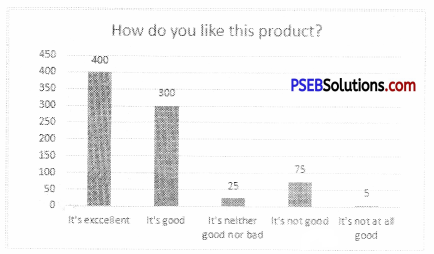
And here I have marked the basic chart elements in Excel each element with different clor for understanding purpose. Most of the time we generally deal with Chart Area, Plot Area, Chart Title, Legends, X-Axis, Y-Axis, Data Labels Data Series, and Gridlines. Here is the pictorial representation of Chart Elements or Chart Objects in Excel:

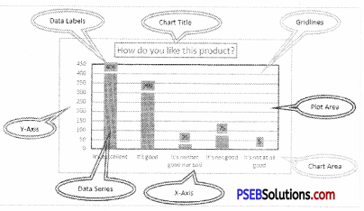
Now will see each element of the Excel Chart in detail :

Chart Area
Chart area in Excel Charts is the largest element (portion) of the Chart. We can format the Chart Area and change its border and background colors to make the charts look more cleaner. Legends, Chart Titles, and Plot Areas are the three major child elements of Chart Area. Generally, we do not change the background color of the charts to make them look more professional. Charts look more cleaner with white or default background color. However, we can change the background color to suit the other parts of the excel sheets to make them consistent.

Basic Elements of Excel Charts – Plot Area
Plot Area is the second-largest element (portion) in Excel Charts. It covers the actual chart data area. We can access the Plot Area and Format it to suit our needs. It is the same as Chart Area, if your project needs different background color then we change it. Otherwise default background color (white) looks more cleaner.

Question 3.
What is Convert Text to Columns? Write down the steps to convert Text to columns.
Answer:
Sometimes we need to separate the contents of one Excel cell into separate columns. For this, you can use the ‘Convert Text to Columns Wizard’.

1. Open the worksheet that contains the text you would like to convert to columns.
2. Select the cells that you would like to convert.
3. On the Data tab, click Text to Columns in the Data Tools group.
4. Choose the format of your current data. Select Delimited if the text contains a character such as a comma, tab, space, or semi-colon to separate the various fields. Otherwise, select Fixed Width if there are a certain number of spaces between each field.
5. A preview of the data in columns appears below, according to the delimiter selected. Click Next.
6. You now need to choose the format for each of the columns. Select the column heading in the Data preview and then select a data type from the column data format options.
7. A preview of your selected data appears below. Click Next.
8. Select the type of character that separates the various fields. You can select as many as are applicable. If you would like to include your own characters that aren’t listed, select the Other checkbox and enter the specific character in the field provided.
9. Once you have selected the data type for each column, click Finish.
10. Your text will now appear in several columns, depending on the number of delimiters in the original list.

Question 4.
What is Data Validation? How to create a Data Validation Rule?
Answer:
Data validation allows you to control exactly what a user can enter into a cell. In our example, we can use data validation to ensure that the user chooses one of the three possible shipping options. To make things even easier, we can insert a drop-down list of the possible options. This kind of data validation allows you to build a powerful, fool-proof spreadsheet. Since users won’t have to type in data manually, the spreadsheet will be faster to use, and there’s a much lower chance that someone can introduce an error.

Data validation in Excel
Since we already have a list of shipping options in the Shipping worksheet, we’re going to tell Excel to use the data in that list to control which values a user can select. But before we do this, we actually need to name the cell range first. Naming cell ranges is one way to keep track of important cell ranges in your spreadsheet.
To create a data validation drop-down list:
Select the cell where you want the drop-down list to appear. In our example, that’s cell E6 on the Invoice worksheet.

1. On the Data tab, click the Data Validation command.
2. A dialog box will appear. In the Allow: field, select List.
3. In the Source: field, type the equals sign (=) and the name of your range, and then click OK. In our example, we’ll type =ShipRange.
4. A drop-down arrow will appear next to the selected cell. Click the arrow to select the desired option. In our example, we’ll select Standard. Alternatively, you can type the shipping option, but Excel will only accept it if it is spelled correctly.
5. The selected value will appear in the cell. Now that we’re searching for the exact name of a shipping option, our VLOOKUP function is working correctly again.

Question 5.
What is Protection? Write down the steps to protect a Worksheet.
Answer:
To prevent a user from accidentally or deliberately changing, moving, or deleting important data from a worksheet or workbook, you can protect Certain worksheet or workbook elements, with or without a password. You can remove the protection from a worksheet as needed.
Protect worksheet elements

1. Select the worksheet that you want to protect.
2. To unlock any cells or ranges that you want other users to be able to change, do the following:

• Select each cell or range that you want to unlock.
• On the Home tab, in the Cells group, click Format, and then click Format Cells.
• On the Protection tab, clear the Locked check box, and then click OK.

3. To hide any formulas that you do not want to be visible, do the following:

• In the worksheet, select the cells that contain the formulas that you want to hide.
• On the Home tab, in the Cells group, click Format, and then click Format Cells.
• On the Protection tab, select the Hidden check box, and then click OK.

4. To unlock any graphic objects (such as pictures, clip art, shapes, or Smart Art graphics) that you want users to be able to change, do the following:

• Hold down CTRL and then click each graphic object that you want to unlock. This displays the Picture Tools or Drawing Tools, adding the Format tab.

5. On the Review tab, in the Changes group, click Protect Sheet.
6. In the Allow all users of this worksheet to list, select the elements that you want users to be able to change.

Question 6.
What is Split Worksheet? Write down the steps to split a worksheet.
Answer:
Split your worksheet to view multiple distant parts of your worksheet at once. To split your worksheet (window) into upper and lower parts (pane), execute the following steps.

1. Click the split box above the vertical scroll bar.
2. Drag it down to split your window.
3. Notice the two vertical scroll bars. For example, use the lower vertical scroll bar to move to row 49. As you can see, the first 6 rows remain visible.
4. To remove the split, double click the horizontal split bar that divides the panes (or drag it up),

PSEB 9th Class Computer Guide MS Excel Part-II Important Questions and Answers

Fill in the Blanks

1. …………….. means to stabilize an object.
(a) Hide
(b) View
(c) Freeze
(d) Pivot
Answer:
(c) Freeze

2. …………….. is a sequence of commands.
(a) Pivot
(b) Macro
(c) Tree
(d) Record.
Answer:
(b) Macro

Short Answer Type Questions

Question 1.
How do I put the password to protect my entire Spreadsheet so data cannot be changed?
Answer:
Perform the followings steps :
1. Click Tools 2. Scroll down to Protection, then Protect Sheet 3. Enter a password, Click OK 4. Re-enter password, Click OK

Question 2.
What is the shortcut to put the filter on data in Microsoft Excel 2013?
Answer:
Ctrl+Shift+L is the shortcut key to s it the filter in data.

Question 3.
What are Freeze Panes and how do I do it?
Answer:
The followings are the steps to perform:
1. Row – Select the row below where you want the split to appear 2. Column – Select the column to the right of where you want the split to appear 3. Go to the Menu Bar 4. Click Windows and then click Freeze Panes.

Question 4.
How do I combine different chart types into my Excel spreadsheet?
Answer:
To combine chart types, follow these steps: 1. If the Chart toolbar isn’t already displayed, right-click any Toolbar and select Chart. 2. On the chart, click the series you want to change. 3. On the Chart toolbar, click the arrow next to the Chart Type button and then select the new chart type for the series (in our example, a line chart).

Question 5.
What is the Ribbon?
Answer:
The ribbon is an area that runs along the top of the application that contains menu items and toolbars available in Excel. The ribbon has various tabs that contain groups of commands for use in the application. The ribbon can be minimized or maximized by pressing CNTRL FI.

Question 6.
What is a Macro in Excel and how would you create an Excel Macro?
Answer:
Excel Macros as sets of instructions that a user records for repetition purposes. Users create macros for repetitive instructions and functions they perform on a regular, basis. To record an Excel macro, you need to select record macro from the developer’s tab and then record the instructions used in the worksheet. Macros can be triggered via a keyboard shortcut.

Question 7.
What is Chart in MS-Excel? Why is it important to you an appropriate chart?
Answer:
The chart is a medium to present the data in graphical visualization, and it is the most important insight of the data. To present the data with perfect visualization and appropriate information, we should always pre-decide on the information to be presented.

As appropriate charts lead to the right decision, it’s necessary to use relevant charts. Refer to the below process chart for appropriate charts :

Question 8.
What is a Dashboard and what are the important things we should keep in mind while creating a dashboard?
Answer:
The dashboard is a technique used to present important information through graphical representation. It is helpful in presenting huge data on a single computer screen so it can be monitored with a glance. There are few things that should be taken care of while preparing the dashboards:

1. Minimum distraction
2. Simple, easy to communicate
3. Important data
4. Few Colors
5. Relevant graphs
6. The dashboard should be on a single computer screen.

Question 9.
How can you format a cell? What are the options?
Answer:
We can format a cell by using the “Format Cells” option and there are 6 options :

1. Number
2. Alignment
3. Font
4. Border
5. Fill
6. Protection

Long Answer Type Questions

Question 1.
Is it possible to make Pivot Table using multiple sources of data? How?
Answer:
Yes, this is possible by using the data modeling technique.
Start with collecting data from various sources :

• Import from a relational database, like Microsoft SQL Server, Oracle, or Microsoft Access. You can import multiple tables at the same time.
• Import multiple tables from other data sources including text files, data feeds, Excel worksheet data, and more. You can add these tables to the Data Model in Excel, create relationships between them, and then use the Data Model to create your Pivot Table.

Question 2.
How to use Data Modeling for creating Pivot Table?
Answer:
After creating relationships between tables, make use of the data for analysis.

• Click any cell on the worksheet
• Click Insert > Pivot Table
• In the Create PivotTable dialog box, under Choose the data that you want to analyze, click Use an external data source
• Click Choose Connection.
• On the Tables tab, in This Workbook Data Model, select Tables in Workbook Data Model.
• Click Open, and then click OK to show a Field List containing all the tables in the Data Model.

Question 3.
What is the IF function in Microsoft Excel?
Answer:
‘If function’ is one of the logical functions in Excel. We use this function to check the logical condition and specify the value whether it’s true or false. ‘If function’ has three arguments but only the first argument is mandatory and the other two are optional.

Question 4.
How can we merge multiple cells’ text strings in a cell?
Answer:
We can merge multiple cells text strings by using the Concatenate function and “&” function.
Example: We have three names: First Name, Middle name, Last name in 3 columns. To merge the names and make it a full name, follow the steps below :
Concatenate Function

• Enter the formula in cell D2
• =CONCATENATE(A2,” “,B2,” “,C2)